Quick start

A worked example

Let’s delve in into the API of Hypertunity by going through a worked example—neural network hyperparameter optimisation. In the following we will tune the number of layers and units, the non-linearity type, as well as the dropout rate and the learning rate of the optimiser.

Disclaimer: This example serves a demonstration purpose only. It does not represent an advanced way of performing neural network architecture search!

First thing we do it to import Hypertunity, tensorflow and numpy and define a helper data loading function:

import hypertunity as ht
import numpy as np
import tensorflow as tf

import hypertunity.reports.tensorboard as ht_tb


def load_mnist():
    (train_x, train_y), (test_x, test_y) = tf.keras.datasets.mnist.load_data()
    data_shape = train_x.shape[1:]
    train_x = train_x.reshape(-1, np.prod(data_shape)).astype(np.float32) / 255.
    mean_train = np.mean(train_x, axis=0)
    train_x -= mean_train
    test_x = test_x.reshape(-1, np.prod(data_shape)).astype(np.float32) / 255.
    test_x -= mean_train
    train_y = tf.keras.utils.to_categorical(train_y, num_classes=10)
    test_y = tf.keras.utils.to_categorical(test_y, num_classes=10)
    return (train_x, train_y), (test_x, test_y)

Next we define a function that will build the model given the architectural hyperparameters and the learning rate, followed by the objective which will wrap the model building and evaluation:

def build_model(inp_size, out_size, n_layers, n_units, p_dropout, activation):
    inp = tf.keras.Input(inp_size)
    h = inp
    for l in range(n_layers - 1):
        h = tf.keras.layers.Dense(n_units, activation=activation)(h)
        h = tf.keras.layers.Dropout(rate=p_dropout)(h)
    h = tf.keras.layers.Dense(out_size, activation=None)(h)
    out = tf.keras.layers.Softmax()(h)
    model = tf.keras.models.Model(inputs=inp, outputs=out)
    return model


def objective_fn(**config) -> float:
    (train_x, train_y), (test_x, test_y) = load_mnist()
    model = build_model(train_x.shape[-1], train_y.shape[-1],
                        config["arch"]["n_layers"],
                        config["arch"]["n_units"],
                        config["arch"]["p_dropout"],
                        config["arch"]["activation"])
    opt = tf.keras.optimizers.Adam(learning_rate=config["opt"]["lr"])
    model.compile(optimizer=opt, loss="categorical_crossentropy")
    model.fit(train_x, train_y, batch_size=100, epochs=1)
    score = model.evaluate(test_x, test_y, batch_size=test_x.shape[0])
    return score

Now that we can build a model, we should define the ranges of possible values for the these parameters. This can be done with creating a Domain instance as follows:

domain = ht.Domain({
    "arch": {
        "n_layers": {1, 3, 5},
        "n_units": {10, 50, 100, 500},
        "p_dropout": [0, 0.9999],
        "activation": {"relu", "selu", "elu"}
    },
    "opt": {
        "lr": [1e-9, 1e-2]
    }
})

The Domain plays a central role in Hypertunity and we will make a frequent use of it later as well. An important related class is the Sample. It can be thought of as one realisation of the variables from the domain, which in our case is one particular configuration of network hyperparameters.

Using the domain, we can set up the optimiser and the result visualiser also used for experiment logging. In this case we use BayesianOptimisation and Tensorboard respectively:

optimiser = ht.BayesianOptimisation(domain)
tb_rep = ht_tb.Tensorboard(domain,
                           metrics=["cross-entropy"],
                           logdir="./mnist_mlp",
                           database_path="./mnist_mlp")

After we create the Tensorboard reporter we will be prompted to run tensorboard –logdir=./mnist_mlp in the console and open Tensorboard in the browser. We can do this also before we launch the actual optimisation.

One last bit before running it is the definition of the job schedule as well as optimiser and reporter update loop. This is to ensure that samples are generated, experiments are run and the results used to improve the underlying model of the BayesianOptimisation optimiser. To schedule one experiment at a time, for 50 consecutive steps we create a Job for each function call of objective_fn with a set of suggested hyperparameters:

n_steps = 50
batch_size = 1
with ht.Scheduler(n_parallel=batch_size) as scheduler:
    for i in range(n_steps):
        samples = optimiser.run_step(batch_size=batch_size, minimise=True)
        jobs = [ht.Job(task=objective_fn, args=s.as_dict() for s in samples]
        scheduler.dispatch(jobs)
        evaluations = [r.data for r in scheduler.collect(n_results=batch_size, timeout=100.0)]
        optimiser.update(samples, evaluations)
        for sample_evaluation_pair in zip(samples, evaluations):
            tb_rep.log(sample_evaluation_pair)

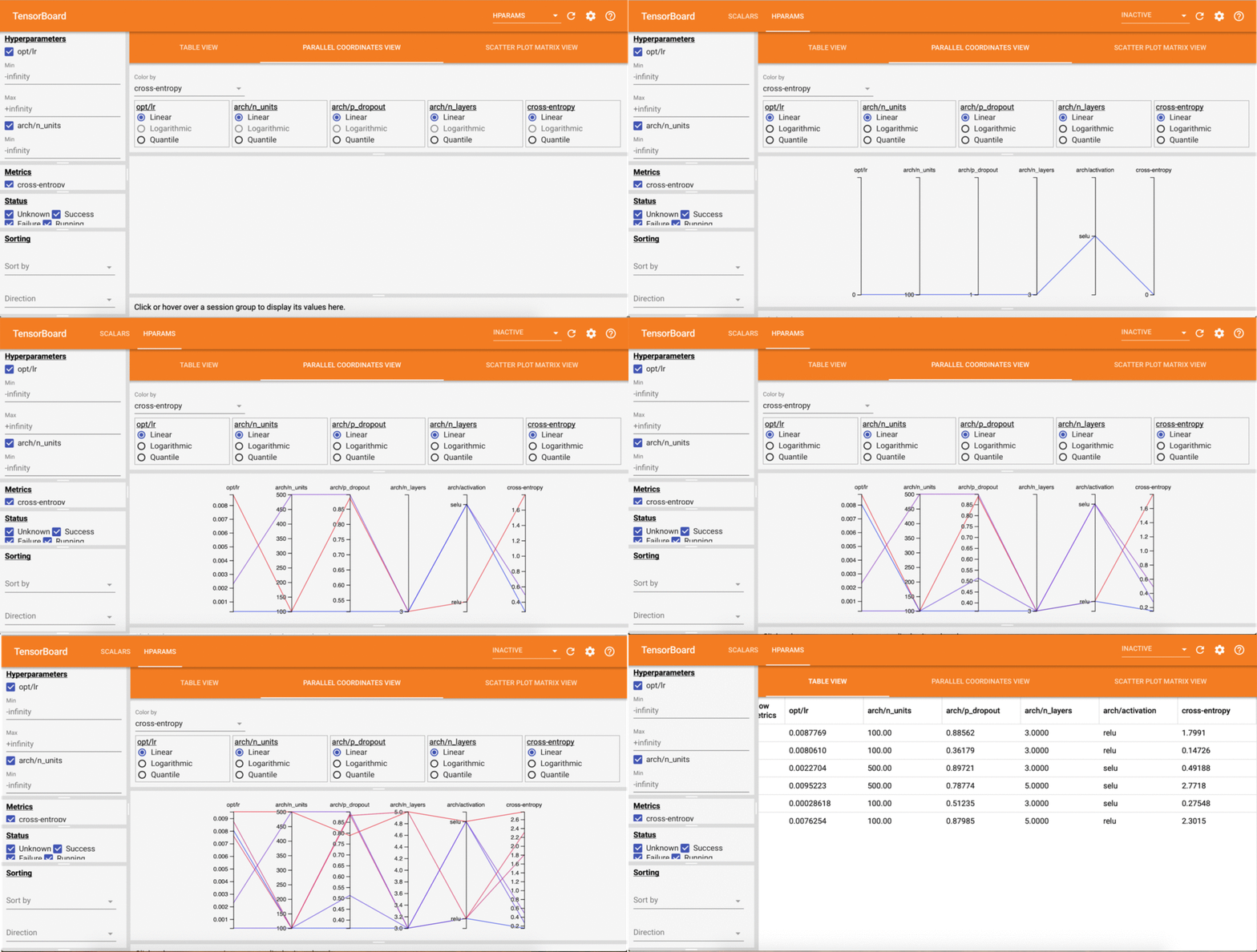
If we have a look at the Tensorboard dashboard while this is running, we should be able to see results being updated live!

Even quicker start

A high-level wrapper class Trial allows for seamless parallel optimisation without having to schedule jobs, update the optimiser or log results explicitly. The API is reduced to the minimum and yet remains flexible as one can specify any optimiser or reporter:

trial = ht.Trial(objective=objective_fn,
                 domain=domain,
                 optimiser="bo",
                 reporter="tensorboard",
                 logdir="./mnist_mlp",
                 database_path="./mnist_mlp",
                 metrics=["cross-entropy"])

trial.run(n_steps, batch_size=batch_size, n_parallel=batch_size)